


Table of Contents
4.1 Motivation and Background
•
Forces play a central role in many hydrodynamic problems.
•
Gravitational acceleration can be cast into force density: .
•
In hydrodynamics, we encounter force densities rather than forces since momentum equation is a PDE for momentum density.
⇒ Forces are momentum density source terms in the Cauchy equation.
Key Applications of Forces in LBM
•
Gravity effects:
◦
Rayleigh-Bénard instability - convection patterns when warmed fluid rises from hot surface.
◦
Rayleigh-Taylor instability - denser fluid descends as lower-density fluid rises.
◦
Gravity waves at free water surface.
•
Other physical problems:
◦
Rotating reference frames subject to radial and Coriolis forces.
◦
Charged or magnetic particles in fluids with electromagnetic fields.
◦
Electrical Double Layer (EDL) effects in electrolytes near charged surfaces.
•
Computational advantages:
◦
In incompressible flows, pressure gradients can be replaced by divergence-free body forces.
◦
Useful in periodic flow configurations (e.g., porous media flows).
◦
Helps avoid accuracy loss from compressibility errors in pressure fields.
•
Additional applications:
◦
Modeling multiphase or multi-component flows.
◦
Fluid-structure interactions via immersed boundary method.
4.2 LBM with Forces in a Nutshell
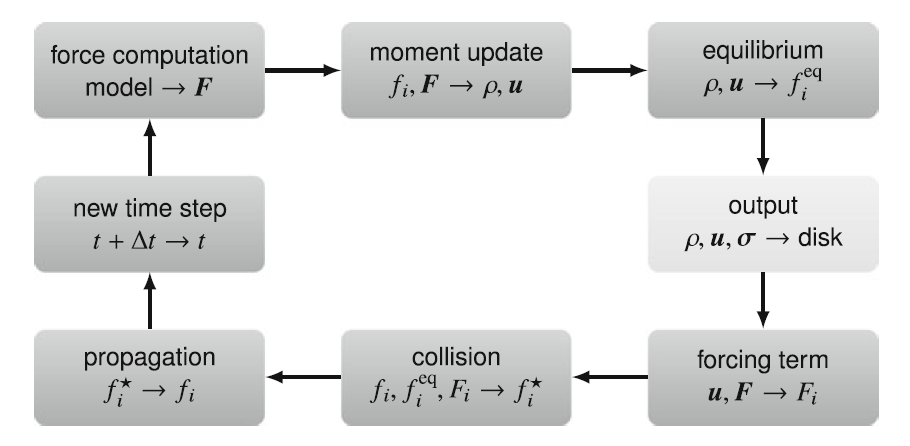
Order of Operations in a Single Time Step (with BGK collision operator)
•
Step 1: Determine force density .
◦
Example: gravity force
•
Step 2: Compute fluid density and velocity:
•
Step 3: Compute equilibrium populations to construct the collision operator:
•
Step 4: Output macroscopic quantities (optional).
◦
Deviatoric stress:
•
Step 5: Compute source term:
◦
Where the source and forcing terms are related as .
•
Step 6: Apply collision and source to find the post-collision populations:
•
Step 7: Propagate populations.
•
Step 8: Increment the time step and go back to Step 1.
Important Remarks
•
The form of the force depends on the underlying physics - not given by LB algorithm.
•
Velocity contains the so-called half-force correction.
◦
Ensures second-order space-time accuracy.
◦
The velocity can be interpreted as the average velocity during the time step, i.e. the average of pre- and post-collision values.
•
Forcing scheme presented here is based on a Hermite expansion (same as Guo et al.). → Alternative forcing schemes exist.
•
Any cyclic permutation of steps permitted with proper initialization.
4.3 Discretisation
4.3.1 Discretisation in Velocity Space
•
Main Question: what is the equivalent polynomial representation in velocity space of the forcing term in the Boltzmann equation?
•
The continuous Boltzmann equation with a forcing term:
◦
Goal: Find discrete velocity structure of forcing term aligned with velocity space discretization of .
◦
Challenge: doesn't appear as isolated term but as:
Mathematical Approach
1.
The Hermite series expansion of the distribution function is:
2.
The derivative property of Hermite polynomials reads:
3.
We can rewrite the Hermite expansion of as follows:
4.
The forcing contribution can be simplified as follows:
Discrete Form
•
Replace continuous with discrete .
•
Rescale velocities: .
•
Renormalize by lattice weights .
•
The discrete form of the forcing term:
•
The discrete velocity Boltzmann equation with a forcing term:
Second-Order Truncation
•
The truncation of the forcing term up to second velocity order (), corresponding to the expansion of :
•
Velocity moments:
◦
Zeroth: (no mass source).
◦
First: (momentum source). → It appears as a body force in the NSE.
◦
Second: (energy source). → a purposefully designed correction to precisely cancel out a spurious error term that arises in the momentum equation of weakly compressible Lattice Boltzmann Methods.
▪
For a incompressible flow:
4.3.2 Discretisation in Space and Time
•
Task consists of two parts:
◦
Advection: Exact via method of characteristics ( ):
◦
Collision with forces: Requires approximation:
First-Order Integration
•
Rectangular discretization:
◦
The integral of collision and forcing terms is approximated by just one point.
•
LBE with force (BGK):
•
Issues:
◦
Only first-order accurate in time.
◦
Cannot absorb errors into viscosity when forces present.
◦
Leads to discrete lattice artifacts.
Second-Order Integration
•
Trapezoidal discretization:
◦
More accurate but time-implicit.
•
Change of variables to recover explicit form:
•
Second-order accurate LBGK with forcing:
◦
Where .
Redefined Macroscopic Moments
•
Density:
•
Velocity:
•
Momentum flux:
4.4 Alternative Forcing Schemes
4.4.1 General Observations
•
Based on the second-order velocity and space-time discretizations, the LBE with a force can be expressed as:
◦
Where is the BGK collision operator and denotes a source, with the forcing given by:
◦
The fluid velocity in the presence of a force is redefined to guarantee the second-order space-time accuracy:
•
The complexity in the LB literature is caused by the fact that:
⇒ There exist different force algorithms that decompose and differently but lead to essentially the same results on the Navier-Stokes level.
•
To generalize the forcing method, the equilibrium velocity can be written as :
◦
: A model-dependent parameter ( for Guo forcing).
•
Equivalence condition:
◦
Schemes equivalent if same up to or .
◦
Valid only for sufficiently small and .
4.4.2 Forcing Schemes
Guo et al. (2002)
•
Based on the Chapman-Enskog analysis.
•
.
◦
Removes undesired derivatives in continuity and momentum equations.
Shan and Chen (1993, 1994)
•
Originally for multi-phase fluids but applicable to single-phase fluids.
•
.
He et al. (1998)
•
Based on near-equilibrium approximation:
•
.
Kupershtokh (2004)
•
Exact difference method → To include the force density in such a way that it merely shifts in velocity space.
•
.
◦
Where and .
◦
The equilibrium for a velocity is directly replaced by the equilibrium for a velocity .
4.5 Chapman-Enskog and Error Analysis in the Presence of Forces
4.5.1 Chapman-Enskog Analysis with Forces
•
In order to be consistent with the remaining terms in the LBE, the forcing term must scale as .
⇒ We should at least have .
•
A hierarchy of -perturbed equations:
•
In the presence of an external force, the hydrodynamic moments are no longer conserved.
⇒ This leads to a redefinition of the solvability conditions for mass and momentum:
◦
The extension to “strengthened” order-by-order solvability conditions reads:
▪
With , which results from .
•
By taking the zeroth and first moments of the equation:
◦
Here, .
•
By taking the zeroth and first moments of the equations :
•
By combining the mass and momentum equations in the and equations:
•
is the contribution responsible for the viscous stress at macroscopic level.
⇒ Therefore, the role of is to remove spurious forcing terms possibly appearing in so that its form is the same as for the force-free case:
◦
The viscous stress is still given by .
•
Finally, we can re-assemble and use and to obtain the correct form of the unsteady NSE with forcing term (up to error terms):
◦
As usual, the dynamic shear and bulk viscosities are and , respectively.
4.5.2 Errors Caused by an Incorrect Force Model
Discretization of Velocity Space: The Issue of Unsteady and Steady Cases
•
Unsteady state:
◦
Term contains the contribution .
⇒ This contribution can be exactly cancelled by , providing the force term is expanded up to the second velocity order.
•
Steady state with standard equilibrium:
◦
Same spurious term is still required as a correction due to the gradient of the velocity .
◦
Still needs second-order expansion.
•
Steady state with incompressible equilibrium:
◦
The steady incompressible NSE is recovered with no spurious terms.
⇒ We must set .
Discretization of Space and Time: The Issue of Discrete Lattice Effects
•
Let us assume a time-dependent process and a forcing term with second-order velocity discretization.
⇒ The macroscopic equations reproduced in this case have the following incorrect form:
◦
First-order time integration errors:
▪
Continuity:
▪
Momentum:
•
Discrete lattice artifacts:
◦
Act on same scale as viscous term ().
◦
Corrupt both mass and momentum equations.
◦
More problematic than velocity discretization errors.
4.6 Boundary and Initial Conditions with Forces
4.6.1 Initial Conditions
•
Equilibrium initialization with forces:
◦
For low-order forcing schemes, where the macroscopic velocity is computed from , the equilibrium initialization is the same as in the force-free case, i.e. .
•
Non-equilibrium initialization with forces (adding the modified non-equilibrium term):
◦
Where
4.6.2 Boundary Conditions
Bounce-Back
•
The principle of the bounce-back rule is not changed by the inclusion of forces.
⇒ Its accuracy does depend on the force implementation.
•
Simple example: a hydrostatic equilibrium where a constant force is balanced by a pressure gradient.
◦
The hydrostatic solution established by the bounce-back rule at boundary node .
◦
Second-order space-time discretization for the bulk dynamics ():
▪
The first factor is positive due to the stability requirement and can be cancelled. → .
◦
First-order space-time discretization for the bulk dynamics ():
▪
The first-orderdiscretization retains discrete lattice artifacts even for constant forces.
Non-Equilibrium Bounce-Back (NEBB)
•
Modified density calculation at wall:
◦
The unknown boundary populations still have to be determined by the bounce-back of their non-equilibrium components.
•
Momentum corrections:
◦
Tangential:
◦
Normal:
•
Unknown populations with forces (top wall example):
4.7 Benchmark Problems
•
Velocity Order:
•
Space-Time Order:
•
Comparing four possible forcing strategies:
Scheme | Velocity Order | Space-Time Order |
I | 1st | 1st |
II | 2nd | 1st |
III | 1st | 2nd |
IV | 2nd | 2nd |
4.7.1 Problem Description
•
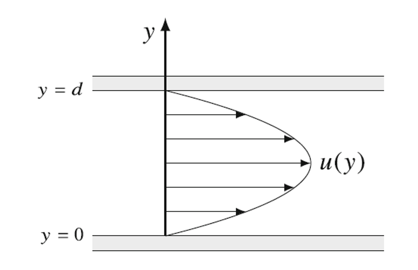
A 2D Poiseuille channel flow driven by a combined pressure gradient and body force :
•
Analytical velocity solution:
◦
Where the no-slip condition () holds at the bottom and top walls ().
4.7.2 Numerical Procedure
•
The BGK collision operator with incompressible equilibrium.
•
The bounce-back and the non-equilibrium bounce-back (NEBB) boundary conditions are tested.
•
Initialization: .
•
Steady-state criterion: between 100 consecutive time steps.
•
Grid: .
MATLAB Code of Poiseuille flow with bounce-back
MATLAB Code of Poiseuille flow with NEBB
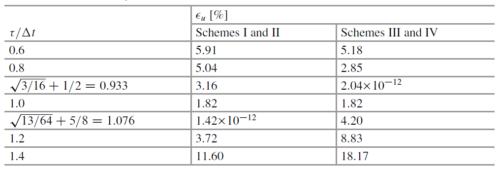
4.7.3 Constant Force
•
A purely force-driven Poiseuille flow: .
•
Using periodic boundary conditions at the inlet and outlet.
•
The force magnitude is (in simulation units).
Results:
•
Bounce-back: Exact solution at specific values.
◦
Schemes I & II: .
◦
Schemes III & IV: .
•
NEBB: Exact for all schemes (no bulk errors for constant force).
4.7.4 Constant Force and Pressure Gradient
•
Combined driving: (in simulation units) → Considering a 50/50 contribution from each term.
•
Using pressure periodic boundary conditions at the inlet and outlet.
Results:
•
Bounce-back: Exact solution at specific values.
◦
Schemes I & II: .
◦
Schemes III & IV: .
▪
Only second-order space-time discretization (Schemes III & IV) maintains physical equivalence.

•
NEBB: Exact for all schemes (no bulk errors for constant force).
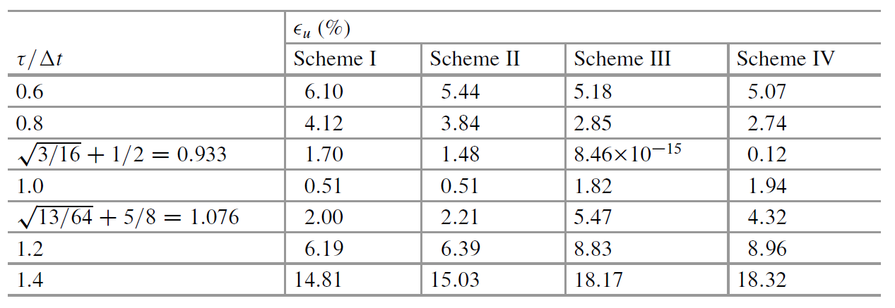
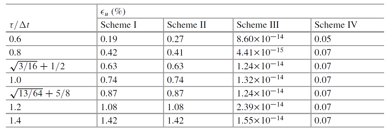
4.7.5 Linear Force and Pressure Gradient
•
The force increases linearly along the streamwise direction.
◦
The total contribution remains constant so that the overall magnitude remains locally (in simulation units) → Considering a 50/50 contribution from each term.
•
The force bulk errors do not vanish any more. → Both bulk and boundary errors can now interfere with the LB solution.
Results:
•
Bounce-back: Only Scheme III achieves exact solution at specific values.
◦
Schemes III: .
◦
First-order velocity discretization required for a steady incompressible flow.
•
NEBB: Only Scheme III achieves exact solution for all values.
◦
Schemes III: the bulk solution free from errors.
◦
-independent boundary treatment.
4.7.6 Role of Compressibility
•
The standard equilibrium recovers the compressible NSE, which approximates incompressible hydrodynamics in the limit of slow flows and small density (pressure) variations.
⇒ Compressibility Errors.
•
The compressibility errors typically have a secondary impact. → They always contaminate the solutions.
◦
For spatially varying forces:
▪
Incompressible equilibrium: First-order velocity discretization optimal.
▪
Standard equilibrium: Second-order slightly better (but differences small).
Key Takeaways
•
Most accurate forcing scheme for general flows: Second-order in both velocity and space-time (Scheme IV).
•
For steady incompressible flows: First-order velocity with second-order space-time (Scheme III).
•
Critical implementation details:
◦
Half-force correction in velocity calculation essential.
◦
Boundary conditions must account for forces.
◦
Initial conditions need force corrections.
•
Error hierarchy: Space-time discretization errors > velocity discretization errors > compressibility errors.
 Go Top of Page