[LBM Study] 2. Analysis of the Lattice Boltzmann Equation

2.1 Chapman-Enskog Analysis

2.1.1 The Perturbation Expansion

•

Key Concept: The distribution function fif_ifi​ is expanded around the equilibrium distribution fieqf_i^\mathrm{eq}fieq​ with Knudsen number Kn\mathrm{Kn}Kn as the expansion parameter: 

f_i = f_i^\mathrm{eq} + \epsilon f_i^{(1)} + \epsilon^2 f_i^{(2)} + \cdots.

◦

where ϵn\epsilon^nϵn is a label indicating the order of Knn\mathrm{Kn}^nKnn.

 Important Assumption: In perturbation analysis, we assume that only the two lowest orders in Kn\mathrm{Kn}Kn are sufficient to find the NSE. 

•

LBE with BGK collision operator: 

f_i(\mathbf{x} + \mathbf{c}_i\Delta t, t + \Delta t) - f_i(\mathbf{x}, t) = -\frac{\Delta t}{\tau}[f_i(\mathbf{x}, t) - f_i^\mathrm{eq}(\mathbf{x}, t)].

•

Mass and Momentum Conservation (Solvability Conditions): 

\sum_i f_i^\mathrm{neq} = 0, \quad \sum_i \mathbf{c}_i f_i^\mathrm{neq} = \mathbf{0}.

•

These can be assumed to hold individually at each order:

\sum_i f_i^{(n)} = 0 \text{ and } \sum_i \mathbf{c}_i f_i^{(n)} = \mathbf{0} \text{ for all } n \geq 1.

2.1.2 Taylor Expansion, Perturbation, and Separation

•

Taylor expanding the LBE gives: 

\Delta t(\partial_t + c_{i\alpha}\partial_\alpha)f_i + \frac{\Delta t^2}{2}(\partial_t + c_{i\alpha}\partial_\alpha)^2f_i + O(\Delta t^3) = -\frac{\Delta t}{\tau}f_i^\mathrm{neq}.

•

After neglecting third and higher order terms and eliminating second-order derivative terms: 

\Delta t(\partial_t + c_{i\alpha}\partial_\alpha)f_i = -\frac{\Delta t}{\tau}f_i^\mathrm{neq} + \Delta t(\partial_t + c_{i\alpha}\partial_\alpha)\frac{\Delta t}{2\tau}f_i^\mathrm{neq}.

•

Expansion of time and space derivatives: 

\Delta t\partial_t f_i = \Delta t\bigl(\epsilon\partial_t^{(1)}f_i + \epsilon^2\partial_t^{(2)}f_i + \cdots \bigl), \quad\quad \Delta t c_{i\alpha} \partial_\alpha f_i = \Delta t\bigl(\epsilon c_{i\alpha}\partial_\alpha^{(1)}f_i \bigl).

•

Separating by orders of Kn\mathrm{Kn}Kn: 

\begin{aligned} O(\epsilon): \quad(\partial_t^{(1)} + c_{i\alpha}\partial_\alpha^{(1)})f_i^\mathrm{eq} = -\frac{1}{\tau}f_i^{(1)}, \\\\ O(\epsilon^2): \quad\partial_t^{(2)}f_i^\mathrm{eq} + (\partial_t^{(1)} + c_{i\alpha}\partial_\alpha^{(1)})(1 - \frac{\Delta t}{2\tau})f_i^{(1)} = -\frac{1}{\tau}f_i^{(2)}. \end{aligned}

2.1.3 Moments and Recombination

•

Equilibrium moments: 

\begin{aligned} \Pi_{\alpha\beta}^{\mathrm{eq}} &= \sum_i c_{i\alpha} c_{i\beta} f_i^{\mathrm{eq}} = \rho u_\alpha u_\beta + \rho c_s^2 \delta_{\alpha\beta},\\\\ \Pi_{\alpha\beta\gamma}^{\mathrm{eq}} &= \sum_i c_{i\alpha} c_{i\beta} c_{i\gamma} f_i^{\mathrm{eq}} = \rho c_s^2 (u_\alpha \delta_{\beta\gamma} + u_\beta \delta_{\alpha\gamma} + u_\gamma \delta_{\alpha\beta}), \\\\ \Pi_{\alpha\beta}^{(1)} &= \sum_i c_{i\alpha} c_{i\beta} f_i^{(1)}. \end{aligned}

•

Taking the 0th to 2nd moments of O(ϵ)O(\epsilon)O(ϵ) Kn\mathrm{Kn}Kn equation yields the O(ϵ)O(\epsilon)O(ϵ) moment equations:

\begin{aligned} \partial_t^{(1)}\rho + \partial_\gamma^{(1)}(\rho u_\gamma) = 0,\\\\ \partial_t^{(1)}(\rho u_\alpha) + \partial_\beta^{(1)}\Pi_{\alpha\beta}^\mathrm{eq} = 0, \\\\ \partial_t^{(1)}\Pi_{\alpha\beta}^\mathrm{eq} + \partial_\gamma^{(1)}\Pi_{\alpha\beta\gamma}^\mathrm{eq} = -\frac{1}{\tau}\Pi_{\alpha\beta}^{(1)}. \end{aligned}

•

Taking the 0th and 1st moments of O(ϵ2)O(\epsilon^2)O(ϵ2) Kn\mathrm{Kn}Kn equation yields the O(ϵ2)O(\epsilon^2)O(ϵ2) moment equations: 

\begin{aligned}\partial_t^{(2)} \rho &= 0, \\\\ \partial_t^{(2)} (\rho u_\alpha) + \partial_\beta^{(1)} \left( 1 - \frac{\Delta t}{2\tau} \right) \Pi_{\alpha\beta}^{(1)} &= 0.\end{aligned}

•

Assembling the mass and momentum equations from their O(ϵ)O(\epsilon)O(ϵ) and O(ϵ2)O(\epsilon^2)O(ϵ2) component equations, we find

\begin{aligned}\left( \epsilon \partial_t^{(1)} + \epsilon^2 \partial_t^{(2)} \right) \rho + \epsilon \partial_\beta^{(1)} (\rho u_\gamma) &= 0, \\\\ \left( \epsilon \partial_t^{(1)} + \epsilon^2 \partial_t^{(2)} \right) (\rho u_\alpha) + \epsilon \partial_\beta^{(1)} \Pi_{\alpha\beta}^{\mathrm{eq}} &= -\epsilon^2 \partial_\beta^{(1)} \left( 1 - \frac{\Delta t}{2\tau} \right) \Pi_{\alpha\beta}^{(1)}.\end{aligned}

◦

Reversing the derivative expansions, these equations become the continuity equation and a momentum conservation equation.

◦

With an as-of-yet unknown viscous stress tensor: 

\sigma_{\alpha\beta} = -\left( 1 - \frac{\Delta t}{2\tau} \right) \Pi_{\alpha\beta}^{(1)}.

 Through Chapman-Enskog analysis, we can finally find Perturbation Moment: 

\Pi_{\alpha\beta}^{(1)} = -\rho c_s^2 \tau \left( \partial_\beta^{(1)} u_\alpha + \partial_\alpha^{(1)} u_\beta \right) + \tau \partial_\gamma^{(1)} (\rho u_\alpha u_\beta u_\gamma).

The second term is an error term arising from the lack of a correct

O(u^3)

term in the equilibrium distribution

f_i^\mathrm{eq}

2.1.4 Macroscopic Equations

•

Final Macroscopic Equations can be obtained by 1) inserting Perturbation Moment Παβ(1)\Pi_{\alpha\beta}^{(1)}Παβ(1)​ into mass and momentum equations from their O(ϵ)O(\epsilon)O(ϵ) and O(ϵ2)O(\epsilon^2)O(ϵ2) component equations, 2) reversing the derivative expansion: 

\begin{aligned}\partial_t \rho + \partial_\gamma (\rho u_\gamma) &= 0, \\\partial_t (\rho u_\alpha) + \partial_\beta (\rho u_\alpha u_\beta) &= -\partial_\alpha p + \partial_\beta \left[ \eta (\partial_\beta u_\alpha + \partial_\alpha u_\beta) \right]\end{aligned}

◦

Pressure: p=ρcs2p = \rho c_s^2p=ρcs2​.

◦

Kinematic viscosity: ν=cs2(τ−Δt2)\nu = c_s^2(\tau - \frac{\Delta t}{2})ν=cs2​(τ−2Δt​).

◦

Dynamic viscosity: η=ρν=ρcs2(τ−Δt2)\eta = \rho \nu = \rho c_s^2(\tau - \frac{\Delta t}{2})η=ρν=ρcs2​(τ−2Δt​).

◦

Bulk viscosity: ηB=23η\eta_B = \frac{2}{3}\etaηB​=32​η.

•

Bulk viscosity differences: 

◦

In monatomic kinetic theory, the bulk viscosity ηB\eta_{B}ηB​ is normally zero.

◦

However, in LBE, the bulk viscosity to be of the order of the shear viscosity η\etaη.

◦

Difference caused by isothermal equation of state usage, fundamentally incompatible with monatomic assumption.

 Stability Condition (for positive viscosity):

•

Necessary condition for stability: τ/Δt≥1/2\tau/\Delta t \geq 1/2τ/Δt≥1/2

•

The same condition was found in the discrete LBGK equation’s behavior;  τ/Δt<1/2\tau / \Delta t < 1/2τ/Δt<1/2 would lead to a divergent under-relaxation.

2.2 Discussion of the Chapman-Enskog Analysis

2.2.1 Dependence of Velocity Moments

•

Third-Order Moment Problem: In standard velocity sets (D2Q9, D3Q19, etc.), third-order moments are not independent: 

\Pi_{xxx}^{eq} = \sum_i c_{ix}^3 f_i^{eq} = \left(\frac{\Delta x}{\Delta t}\right)^2 \sum_i c_{ix} f_i^{eq} = \left(\frac{\Delta x}{\Delta t}\right)^2 \Pi_x^{eq}.

◦

This results in O(u3)O(u^3)O(u3) errors in the macroscopic momentum equation (stress tensor).

2.2.2 Time Scale Interpretation

•

Common Misinterpretation: 

∂_t=ϵ∂_t^{(1)}+ϵ^2∂_t^{(2)}+⋯.

◦

Time derivative expansion is often misinterpreted as a decomposition into different time scales. → Viewed as "clocks ticking at different speeds".

◦

This interpretation can lead to false conclusions.

•

Example: Steady Poiseuille Flow

◦

Steady Poiseuille flow: ∇p=∇⋅σ\nabla p = \nabla \cdot \sigma∇p=∇⋅σ (pressure gradient balanced by viscous stress).

◦

Correct physics: ∂t(uα)=0\partial_t(u_\alpha) = 0∂t​(uα​)=0 (velocity doesn't change with time).

◦

False conclusion from time scale interpretation:

▪

∂t(1)(uα)=0\partial_t^{(1)}(u_\alpha) = 0∂t(1)​(uα​)=0 and ∂t(2)(uα)=0\partial_t^{(2)}(u_\alpha) = 0∂t(2)​(uα​)=0 independently. → This would lead to: ∇p=0\nabla p = 0∇p=0 and ∇⋅σ=0\nabla \cdot \sigma = 0∇⋅σ=0 separately.

▪

Result: No flow at all! (contradicts physical reality).

◦

Correct Understanding:

▪

∂t(n)∂_t^{(n)}∂t(n)​ are NOT actual time derivatives. → They are perturbation expansion terms at different orders in ϵ\epsilonϵ. → Only their sum equals the physical time derivative!

▪

Correct relation: ∂t(uα)=∂t(1)(uα)+∂t(2)(uα)=0.\partial_t(u_\alpha) = \partial_t^{(1)}(u_\alpha) + \partial_t^{(2)}(u_\alpha) = 0.∂t​(uα​)=∂t(1)​(uα​)+∂t(2)​(uα​)=0.

▪

This gives: ∇p=∇⋅σ\nabla p = \nabla \cdot \sigma∇p=∇⋅σ (physically correct balance).

2.3 Alternative Equilibrium Models

2.3.1 Linear Fluid Flow

•

Discrete Equilibrium Distribution:

f_i^{\mathrm{eq}} = w_i ρ \left( 1 + \frac{\mathbf{c}_i \cdot \mathbf{u}}{c_s^2} + \frac{(\mathbf{c}_i \cdot \mathbf{u})^2}{2c_s^4} - \frac{\mathbf{u} \cdot \mathbf{u}}{2c_s^2} \right) = w_i ρ \left( 1 + \frac{c_{iα} u_α}{c_s^2} + \frac{u_α u_β (c_{iα} c_{iβ} - c_s^2 δ_{αβ})}{2c_s^4} \right).

•

Linearized Equilibrium Distribution (used in acoustics): 

f_i^\mathrm{eq} = w_i\left(\rho + \rho_0\frac{c_{i\alpha}u_\alpha}{c_s^2}\right).

◦

ρ0\rho_0ρ0​: the rest state density.

•

This produces linearized macroscopic equations (Chapman-Enskog analysis results): 

\begin{aligned} \partial_t \rho + \rho_0 \partial_\alpha u_\alpha = 0, \\\\ \rho_0 \partial_t u_\alpha = -\partial_\alpha p + \eta \partial_\beta \left( \partial_\beta u_\alpha + \partial_\alpha u_\beta \right). \end{aligned}

◦

Pressure: p=ρcs2p = \rho c_s^2p=ρcs2​.

◦

Dynamic shear viscosity: η=ρ0cs2(τ−Δt/2)\eta = \rho_0 c_s^2 (\tau - \Delta t/2)η=ρ0​cs2​(τ−Δt/2).

2.3.2 Incompressible Flow

•

Incompressible Equilibrium Distribution:

◦

Using the fact that ρ′/ρ0=O(Ma2)\rho'/\rho_0 = O(Ma^2)ρ′/ρ0​=O(Ma2) in steady flow: 

f_i^\mathrm{eq} = w_i\rho + w_i\rho_0\left(\frac{c_{i\alpha}u_\alpha}{c_s^2} + \frac{u_\alpha u_\beta(c_{i\alpha}c_{i\beta} - c_s^2\delta_{\alpha\beta})}{2c_s^4}\right).

•

This recovers the exact incompressible Navier-Stokes equations in steady state.

2.4 Stability

2.4.1 Stability Analysis

•

Courant number insufficient for LBM:
⇒ Unlike standard CFD where C=∣u∣ΔtΔx≤1C = \frac{|u|\Delta t}{\Delta x} \leq 1C=Δx∣u∣Δt​≤1 often determines stability, LBM has additional degrees of freedom (relaxation times) that make Courant number alone inadequate.

•

LBM stability analysis requires inversion of q×qq \times qq×q matrix (where qqq is number of populations) due to one equation per velocity direction ci\mathbf{c}_ici​, making it more complex than standard CFD.

•

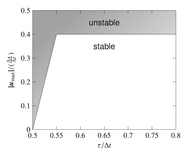
Stability map exists: ∣u∣max⁡(τ)|u|_{\max}(\tau)∣u∣max​(τ) defines maximum achievable velocity magnitude for given relaxation time τ\tauτ before instability sets in.

◦

High Reynolds number dilemma: for Re=∣u∣NΔxνRe = \frac{|u|N\Delta x}{\nu}Re=ν∣u∣NΔx​, achieving high ReReRe requires compromise between maximum velocity and minimum viscosity, both constrained by stability limits.

2.4.2 BGK Stability

•

Stability Conditions for BGK Collision Operator:

◦

Sufficient stability condition is the non-negativity of all equilibrium populations. → τ/Δt>1/2τ/Δt > 1/2τ/Δt>1/2 & fieq≥0f_i^\mathrm{eq} \ge 0fieq​≥0 for all iii

◦

Since the equilibrium populations are functions of the velocity u\mathbf{u}u, this can be expressed as a sufficient stability condition for the velocity u\mathbf{u}u.

▪

For D2Q9D2Q9D2Q9, D3Q15D3Q15D3Q15, D3Q19D3Q19D3Q19, D3Q27D3Q27D3Q27: 

|\mathbf{u}_\mathrm{max}| < \sqrt{\frac{1}{3}}\frac{\Delta x}{\Delta t} \approx 0.577\frac{\Delta x}{\Delta t}.

◦

 Optimal stability condition is the non-negativity of the rest equilibrium population. → τ/Δt>1τ/Δt > 1τ/Δt>1 & f0eq>0f_0^\mathrm{eq} \gt 0f0eq​>0

◦

Velocity magnitude condition: 

|\mathbf{u}| < \sqrt{\frac{2}{3}}\frac{\Delta x}{\Delta t}.

 Stability in Practical Simulations: 

•

In real simulations with boundaries, as τ/Δtτ/Δtτ/Δt → 12\frac{1}{2}21​, ∣umax∣|u_\mathrm{max}|∣umax​∣ should approaches zero: 

|\mathbf{u}_\mathrm{max}|(\tau) = 8\left(\frac{\tau}{\Delta t} - \frac{1}{2}\right)\frac{\Delta x}{\Delta t} \quad\quad \text{ for } \quad \frac{\tau}{\Delta t} < 0.55.

•

As a guideline to find stable parameters for small viscosities:

◦

Start with the sufficient stability condition for all τ/Δt>12.\tau / \Delta t > \frac{1}{2}.τ/Δt>21​.

◦

If simulations are unstable, then perform a few simulations with different values of τ\tauτ and u\mathbf{u}u to find an empirical relation ∣umax∣(τ)|u_\mathrm{max}|(\tau)∣umax​∣(τ).

2.4.3 Stability for Advanced Collision Operators

•

TRT (Two-Relaxation-Time) Model
⇒ In the TRT framework, there is a certain combination of τ+\tau^+τ+ and τ−\tau^-τ− that governs the stability and accuracy of simulations: 

\Lambda = \left(\frac{\tau^+}{\Delta t} - \frac{1}{2}\right)\left(\frac{\tau^-}{\Delta t} - \frac{1}{2}\right).

◦

A recommended choice is Λ=1/4\Lambda=1/4Λ=1/4. → This corresponds to τ/Δt=1\tau / \Delta t = 1τ/Δt=1 in the BGK case, and allows the same optimal stability from which the velocity condition in ∣u∣<2/3ΔxΔt|\mathbf{u}| < \sqrt{2/3}\Delta x \Delta t∣u∣<2/3​ΔxΔt.

◦

For any valude of τ+\tau^+τ+, one can always select the free parameter τ−\tau^-τ− such that Λ=1/4\Lambda=1/4Λ=1/4.

◦

The advantage of the TRT model is therefore that the stability condiiton and the kinematic viscosity ν=cs2(τ−Δt2)\nu = c_s^2(\tau - \frac{\Delta t}{2})ν=cs2​(τ−2Δt​) are decoupled.

2.4.4 Stability Improvement Guidelines

•

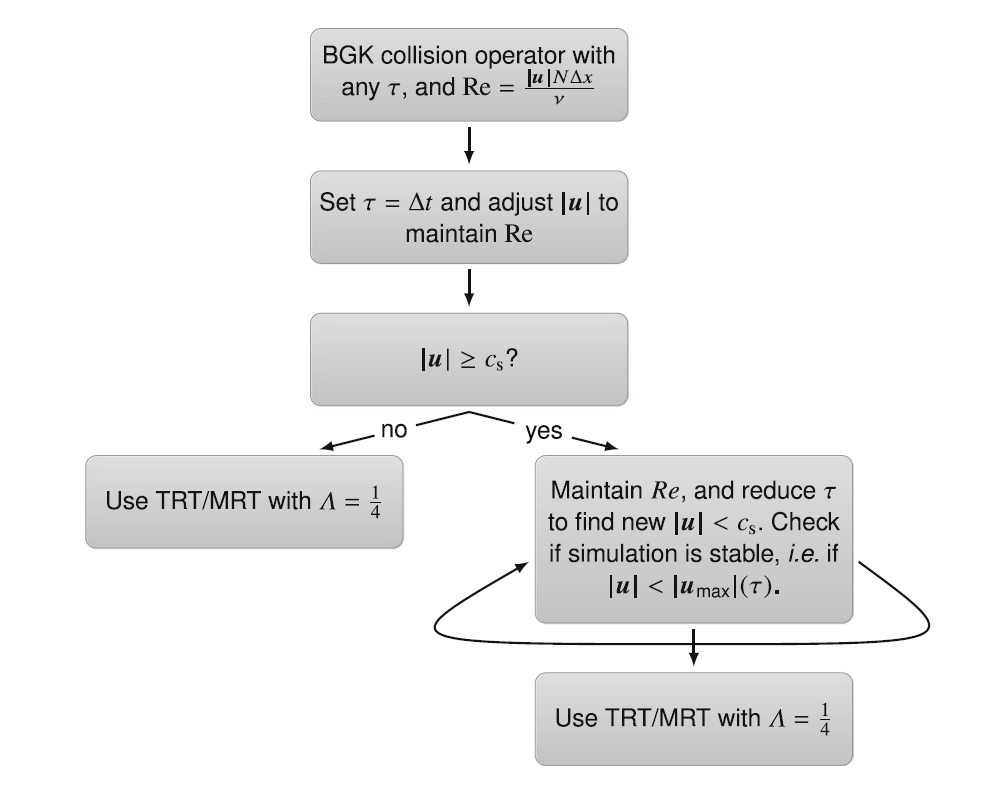
Stability Improvement Process:

Start with BGK collision operator with any τ\tauτ and Reynolds number Re\text{Re}Re: 

\text{Re} = \frac{|u|N\Delta x}{c_s^2\left(\tau - \frac{\Delta t}{2}\right)}.

•

NNN is the number of lattice nodes along a characteristic length scale l=NΔxl=N \Delta xl=NΔx.

Set τ=Δt\tau = \Delta tτ=Δt and adjust ∣u∣|\mathbf{u}|∣u∣to matchthe Reynolds number.

Check if ∣u∣≥cs|\mathbf{u}| ≥ c_s∣u∣≥cs​:

•

If No → Check if simulation is stable.

•

If Yes → Maintain Re\text{Re}Re, reduce τ\tauτ to find new ∣u∣＜cs|\mathbf{u}| ＜ c_s∣u∣＜cs​.
                Check if ∣u∣<∣umax∣(τ)|\mathbf{u}| < |\mathbf{u}_\mathrm{max}|(\tau)∣u∣<∣umax​∣(τ).

If unstable → Use TRT/MRT with Λ = 1/4.

2.5 Accuracy

2.5.1 Formal Order of Accuracy

•

Truncation error analysis through Taylor expansion is used: 

∂u/∂t - ν(∂²u/∂y²) = (Δt/2)(∂²u/∂t²) + ν(Δy²/4!)(∂⁴u/∂y⁴) + O(Δt²) + O(Δy⁴).

◦

This demonstrates the scheme is first-order in time and second-order in space.

2.5.2 Accuracy Measurement

•

L₂ Error Norm: 

\epsilon_q(t) := \sqrt{\frac{\sum_\mathbf{x}[q_n(\mathbf{x},t) - q_a(\mathbf{x},t)]^2}{\sum_\mathbf{x} q_a^2(\mathbf{x},t)}}.

2.5.3 Numerical Errors

Error Type	Description	Mitigation
Round-off Error	Due to finite precision	Use double precision
Iterative Error	Incomplete convergence	Convergence criterion: ε < 10 ⁻ ⁷
Discretization Error	Main error from discretizing PDEs	Can be controlled through τ selection

2.5.4 Modeling Errors

•

O(u3)O(u^3)O(u3) error:

◦

Due to insufficient isotropy of standard lattices.

◦

Negligible when Ma2≪1\text{Ma}^2 ≪ 1Ma2≪1.

•

Compressibility error:

◦

O(Ma2)O(\text{Ma}^2)O(Ma2) magnitude.

◦

Difference from incompressible NSE.

2.5.5 Lattice Boltzmann Accuracy

•

Optimization Conditions:

Condition	BGK τ/Δt	TRT Λ	Application
Cancel O(ε ³)	≈ 0.789	1/12	Advection-dominated
Cancel O(ε ⁴)	≈ 0.908	1/6	Diffusion-dominated
Optimal stability	1.0	1/4	General cases

2.5.6 Accuracy Improvement Guidelines

•

Primary Objective:

◦

Optimize accuracy while respecting non-dimensional groups of the problem.

◦

Match non-dimensional numbers (Reynolds number, Péclet number) between physical problem and LB scheme.

•

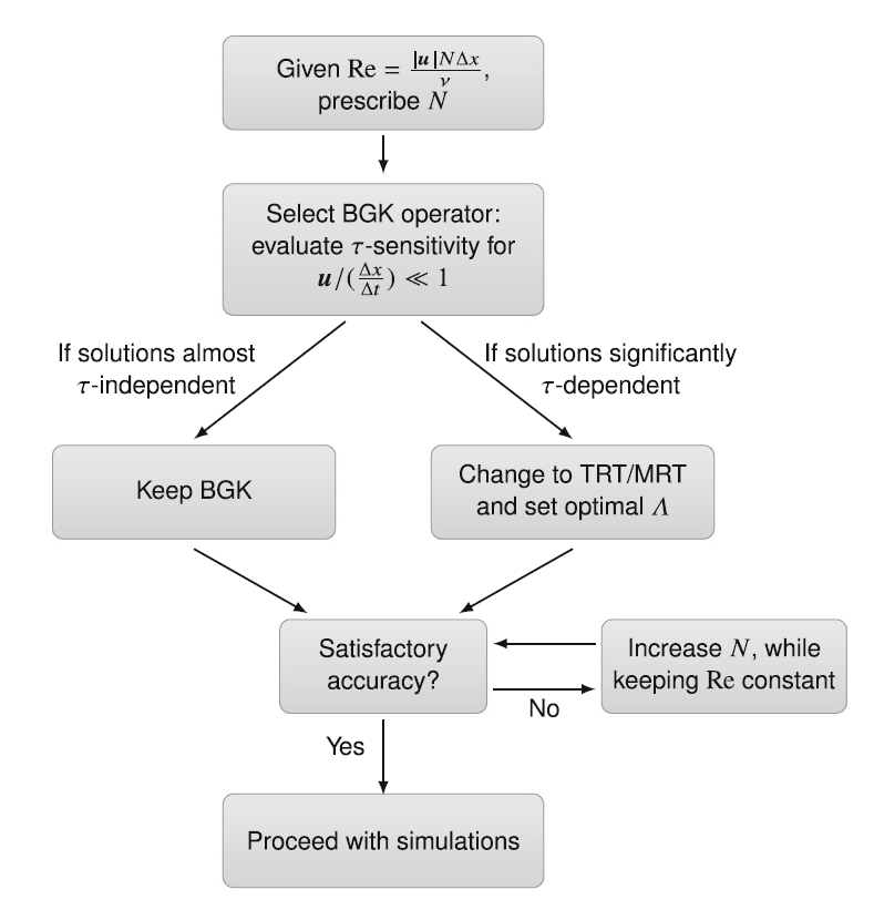
Accuracy Improvement Process:

Initial Setup and Parameter Selection

Determine relevant non-dimensional numbers (Reynolds number).

Select grid number NNN based on computational resources.

Set final parameter τ\tauτ as main control variable.

Collision Operator Assessment and Selection

Start with BGK collision operator.

Evaluate τ\tauτ-sensitivity for velocity condition: 

\mathbf{u} / \big( \frac{Δx}{Δt} \big) ≪ 1.

Keep BGK if solutions almost τ\tauτ-independent 
or Change to TRT/MRT if significantly τ\tauτ-dependent.

Accuracy Optimization and Final Adjustment

Assess current accuracy satisfaction.

If unsatisfactory → Increase grid number NNN while keeping Reynolds number constant.

Proceed with simulations using optimized parameters.

2.6 Summary

Key Points

•

Chapman-Enskog analysis: Establishes connection between LBE and macroscopic NSE.

•

Macroscopic equations: LBE solves weakly compressible NSE, converging to incompressible NSE as Ma2→0Ma² → 0Ma2→0.

•

Stability: τ>Δt/2τ > Δt/2τ>Δt/2 is essential condition, with more stringent constraints in practice.

Practical Recommendations

High Reynolds number simulations: Use TRT/MRT recommended.

Accuracy optimization: Choose τ\tauτ or Λ\LambdaΛ based on problem characteristics.

Stability issues: Set τ=Δtτ = Δtτ=Δt then adjust velocity.

Minimize compressibility error: Maintain Ma<0.1Ma < 0.1Ma<0.1.

Go Top of Page