


Table of Contents
1.1 Introduction
•
If we can solve the Boltzmann equation numerically, this may also indirectly give us a solution to the Navier-Stokes Equation (NSE).
•
The numerical scheme for the Boltzmann equation somewhat paradoxically turns out to be quite simple, both to implement and to parallelise.
◦
A simple hyperbolic equation which essentially describes the advection of the distribution function with the particle velocity .
◦
The ource term depends only on the local value of and not on its gradients.
1.2 The Lattice Boltzmann Equation in a Nutshell
1.2.1 Overview
•
The basic quantity of the Lattice Boltzmann Method (LBM) is the discrete-velocity distribution function .
◦
It represents the density of particles with velocity at position and time .
◦
Mass density and momentum density can be expressed as:
•
The time step and lattice spacing respectively represent a time resolution and a space resolution in any set of units.
◦
The most common choice in the LB (Lattice Boltzmann) literature is lattice units → and .
◦
We can convert quantities between lattice units and physical units. → Law of Similarity: only ensure that the relevant dimensionless numbers.
•
The discrte velocities and weighting coefficients form velocity sets .
◦
Different velocity sets are used for different purposes.
◦
These velocity sets are usually denoted by , where is the number of spatial dimensions the velocity set covers and is the set’s number of velocities.
◦
Commonly used velocity sets: , , , , and . → In 3D, the most commonly used velocity set is .
•
In the basic isothermal LBE (Lattice Boltzmann Equation), determines the relation between pressure and density .
◦
Because of this relation, it can be shown that represents the isothermal model’s speed of sound.
◦
In all the velocity sets, this constant is .
•
By discretising the Boltzmann equation in velocity space, physical space, and time, we find the LBE:
◦
This expresses that particles move with velocity to a neighbouring point at the next time step .
◦
At the same time, particles are affected by a collision operator .

•
The simplest collision operator that can be used for Navier-Stokes simulations is the BGK (Bhatnagar-Gross-Krook) operator:
◦
It relaxes the populations towards an equilibrium at a rate determined by the relaxation time .
◦
This equilibrium is given by:
◦
The equilibrium is such that its moments are the same as those of , i.e. and .
◦
The equilibrium depends on the local quantities density and fluid velocity only.
•
The link between the LBE and the NSE can be determined using the Chapman-Enskog analysis.
◦
The LBE results in macroscopic behaviour according to the NSE, with the kinematic shear viscosity given by the relaxation time as:
◦
The kinematic bulk viscosity given as
1.2.2 The Time Step: Collision and Streaming
•
The Lattice BGK (LBGK) equation reads:
◦
We can decompose this equation into two distinct parts: Collision (or Relaxation) & Streaming (or Propagation).
•
The first part is collision:
◦
represents the distribution function after collisions
◦
is found from:
◦
If →
•
The second part is streaming:
•
Overall, the LBE concept is straightforward.
◦
Collision: one calculates the density and the macroscopic velocity to find the equilibrium distributions and the post-collision distribution .
◦
Streaming: we stream the resulting distribution to neighbouring nodes.
1.3 Implementation of the Lattice Boltzmann Method in a Nutshell
1.3.1 Initialization
•
The simplest approach to initializing the populations at the start of a simulation is to set them to:
via:
•
Often, the values and are used.
1.3.2 Time Step Algorithm
•
The core LBM algorithm consists of a cyclic sequence of substeps, with each cycle corresponding to one time step.

◦
The dark grey boxes show sub-steps that are necessary for the evolution of the solution.
◦
The light grey box indicates the optional output step.
◦
The pale boxes indicate steps with details provided in later sections (Boundary Conditions & Forces).
1.
Compute the macroscopic moments and from via:
2.
Obtain the equilibrium distribution from:
3.
If desired, write the macroscopic fields , , and/or to the hard disk for visualisation or post-processing. The viscous stress tensor can be computed from:
4.
Perform collision (relaxation) as shown in:
5.
Perform streaming (propagation) via:
6.
Increase the time step, setting to , and go back to step 1 until the last time step or convergence has been reached.
1.3.3 Notes on Memory Layout and Coding Hints
•
Initialisation
◦
In a 2D simulation,
▪
Macroscopic fields (2D arrays) → , ,
▪
Populations (3D array) →
▪
and are the number of lattice nodes in x- and y-directions and is the number of velocities.
•
Streaming
◦
The streaming step must be implemented carefully to prevent overwriting population data before it has been streamed from the source node.
◦
Three common strategies exist to handle this:
1.
Opposite-Direction Sweep: Use a temporary buffer for a single population while sweeping through memory in the direction opposite to streaming.
•
Helper functions like circshift (Matlab), numpy.roll (Python), and CSHIFT (Fortran) can simplify this approach.
2.
Two-Array (Swap) Method: Allocate two full population arrays (, ).
•
Read from and write the streamed populations to .
3.
Combined Stream-and-Collide: Perform streaming and collision in a single, fused step.
•
This reads required populations from adjacent nodes directly into the collision calculation at the current node.
•
Updating Macroscopic Variables
◦
Instead of using loops, unroll the summations for calculating macroscopic moments like density and velocity . → Increase the CPU’s computing efficiency.
◦
For the velocity set, the unrolled implementations would be:
•
Equilibrium
◦
It is recommended to unroll the loops for the equilibrium computation ( ), writing separate expressions for each direction of the distributions.
◦
Pre-calculate constants to avoid expensive divisions inside the main loop ( , ).
•
Collision
◦
To optimize the collision step , pre-calculate the relaxation frequency.
▪
Define constants like and once before the main loop.
▪
The collision step then becomes a more efficient calculation: .
1.4 Discretization in Velocity Space
1.4.1 Non-Dimensionalization
•
To simplify the derivation, the governing equations are non-dimensionalized.
•
The continuous and force-free Boltzmann equation in its non-dimensional form is:
◦
: Particle distribution function.
◦
: Components of the spatial coordinate vector .
◦
: Components of the particle velocity vector .
◦
: Collision operator.
•
The corresponding non-dimensional equilibrium distribution function is:
◦
: Equilibrium distribution function.
◦
: Non-dimensional temperature.
◦
: Number of spatial dimensions.
1.4.2 Hermite Polynomials
•
Hermite Polynomials (HPs) are used for the discretization of integrals and form the mathematical basis of the Hermite series expansion.
•
They are a set of orthogonal polynomials constructed from a Gaussian weight function .
•
The multidimensional HP of rank is defined as:
◦
: Hermite Polynomial tensor of rank .
◦
: Gaussian weight function.
◦
: th order gradient operator.
1.4.3 Hermite Series Expansion of the Equilibrium Distribution
•
The equilibrium distribution function is expanded into an infinite Hermite series.
◦
A key insight is that the expansion coefficients are directly related to the macroscopic moments of the fluid (density, momentum, energy, etc.).
•
The equilibrium distribution function has the same mathematical form as the Hermite weight function , allowing it to be expressed as:
◦
: The equilibrium distribution function.
◦
: Macroscopic density.
◦
: Macroscopic velocity.
◦
: Non-dimensional temperature.
◦
: Particle velocity vector.
◦
: Number of spatial dimensions.
◦
: The Hermite weight function (a Gaussian).
•
Key Conclusion: To recover the correct macroscopic conservation laws for hydrodynamics, it is sufficient to truncate the Hermite series expansion after the second-order term.
◦
This is a crucial simplification that makes the LBM computationally feasible.
1.4.4 Discretisation of the Equilibrium Distribution Function
•
The Gauss-Hermite quadrature rule is used to replace continuous integrals over velocity space with discrete, weighted sums.
⇒ This rule allows for the exact integration of polynomials by sampling them at a few specific points called abscissae .
•
To obtain velocity sets with simple integer components, the abscissae are rescaled to define the discrete particle velocities :
•
This procedure yields the final form of the discrete equilibrium distribution function. This equation is a cornerstone of the LBM, shown here for an isothermal () system:
◦
The Greek letters and are indices representing the Cartesian coordinate components ( , , ).
▪
The Einstein summation convention is applied. → (the vector dot product).
▪
is the Kronecker delta, which is 1 if and 0 if .
◦
: The discrete equilibrium distribution for the th velocity direction.
◦
: The lattice weight associated with direction .
◦
: The macroscopic fluid density.
◦
: The macroscopic fluid velocity vector ( and are its components).
◦
: The discrete velocity vector for direction ( and are its components).
◦
: The lattice speed of sound, a constant determined by the velocity set.
1.4.5 Discretisation of the Particle Distribution Function
•
The same discretization process used for the equilibrium function is now applied to the non-equilibrium particle distribution function .
◦
This projects the continuous function onto the discrete velocity set , resulting in a finite set of populations .
◦
These populations become the fundamental variables of the LBM.
•
The evolution of these discrete populations is governed by the discrete-velocity Boltzmann equation:
◦
: The discrete particle distribution (or population) for direction at position and time .
◦
: The component of the discrete velocity . The repeated implies summation over all spatial components.
◦
: The discrete collision operator acting on the th population.
•
A major consequence of this discretization is that macroscopic quantities are now computed through simple, computationally efficient summations over the discrete populations:
1.4.6 Discretisation of the Particle Distribution Function
•
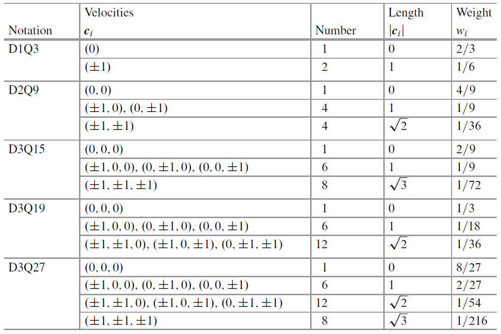
A key component of the Lattice Boltzmann Method is the choice of the discrete velocity set and its corresponding weights .
•
General Comments and Definitions
◦
Velocity sets are commonly named using the notation, where is the number of spatial dimensions and is the number of discrete velocities.
◦
Implementation Warning: The numbering of velocity vectors (”” vs. ””) is not consistent across the literature.
◦
Here follows the convention of using index for the rest velocity () if one exists.
•
Construction and Requirements of Velocity Sets
◦
To correctly solve the NSE, a velocity set and its weights must satisfy certain isotropy conditions.
◦
The key conditions are:
◦
Additional Constraints for Standard LBM:
▪
All weights must be non-negative: .
▪
For simple streaming on a uniform grid, the velocity components are typically integer multiples of .
⇒ In lattice units where and , the velocity vectors have integer components.
•
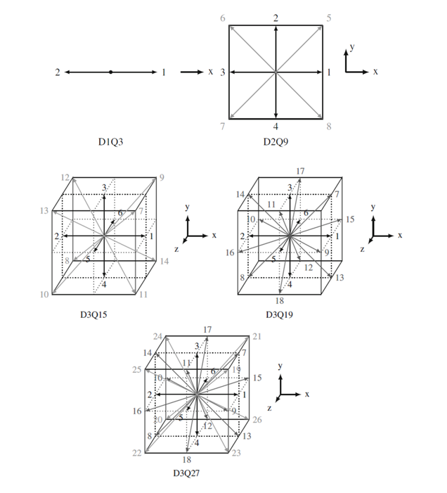
Common Velocity Sets for Hydrodynamics
◦
The most common velocity sets used for hydrodynamic simulations are , , , , and .
◦
Practical Guidance for 3D Simulations:
▪
is generally a good compromise for simulating laminar flows.
▪
offers better rotational invariance and is preferred for high Reynolds number or turbulent flows, although it is more computationally expensive.
•
Equilibrium Distributions
◦
To improve computational performance, it is highly recommended to use the "unrolled" form of the equilibrium equation for each direction rather than calculating it in a loop.
◦
Example for (using and in lattice units):
•
Macroscopic Moments
◦
The velocity sets are designed such that the moments of the equilibrium distribution can be expressed simply in terms of macroscopic variables.
⇒ These relations are fundamental to the Chapman-Enskog analysis that proves the LBM-to-NSE correspondence.
◦
The key equilibrium moments are:
1.5 Discretization in Space and Time
1.5.1 Method of Characteristics
•
Core Idea:
◦
The method transforms the partial differential equation (PDE) for the discrete populations into a simpler ordinary differential equation (ODE) that is valid along specific trajectories in spacetime, known as "characteristics."
•
Starting Equation:
◦
The starting point is the discrete-velocity Boltzmann equation.
◦
: The discrete population for direction .
◦
: The discrete velocity vector for direction ( is its component).
◦
: The discrete collision operator.
•
The Transformation to an ODE (The Characteristic Trajectory):
◦
The advection operator on the left , is converted into a total derivative along a characteristic trajectory defined by:
◦
This simplifies the original PDE to an ODE along this trajectory:
•
The Integral Form (Key Result):
◦
By integrating the ODE along the characteristic trajectory over a single time step from to , we obtain the integral form of the LBE.
◦
The integration of the left-hand side is exact, according to the fundamental theorem of calculus.
◦
The resulting equation, generalized for any arbitrary starting point is:
◦
This equation is central because it reveals the discretization pattern:
1.
Left-hand side: An exact, discrete update rule for propagation, showing that during a time step , the population moves from to .
2.
Right-hand side: An integral of the collision term along the trajectory, which must be approximated in subsequent steps.
1.5.2 First- and Second-Order Discretization
•
First-Order Discretization
◦
The simplest approximation uses a first-order (rectangular) rule, which evaluates the collision operator at the beginning of the time step .
◦
This approximation of the integral results in the explicit discretized LBE:
•
Second-Order Discretization
◦
A more accurate approximation uses the second-order trapezoidal rule to evaluate the collision integral:
◦
This scheme is initially implicit because the collision term at time depends on the unknown populations at that same time.
◦
However, through a specific change of variables (), this implicit equation can be transformed into an explicit equation that has the same form as the one derived from the first-order rule.
•
The fact that the second-order accurate trapezoidal scheme can be rewritten into the same form as the first-order scheme proves that the standard LBE is second-order accurate in time.
1.5.3 BGK Collision Operator
•
To complete the LBE, the collision operator must be specified.
⇒ The simplest and most widely used choice is the Bhatnagar-Gross-Krook (BGK) model, also known as the single-relaxation-time (SRT) model.
•
Definition
◦
The BGK operator models the complex process of particle collisions as a simple linear relaxation of each population towards its corresponding local equilibrium state :
◦
: The discrete particle population for direction .
◦
: The discrete equilibrium population.
◦
: A characteristic time scale known as the relaxation time, which controls the rate of equilibration.
•
The Lattice BGK (LBGK) Equation
◦
Substituting the BGK operator into the discretized LBE (first-order discretization) yields the full Lattice BGK (LBGK) equation:
◦
This simple form is capable of reproducing the full Navier-Stokes equations, which is a primary reason for the popularity of the LBM.
◦
Note on Accuracy and Other Operators:
▪
Although the LBGK equation above can be derived from a first-order time integration, it is actually second-order accurate in time.
▪
More advanced operators like the Two-Relaxation-Time (TRT) and Multiple-Relaxation-Time (MRT) models exist to overcome some of its limitations.
•
Relaxation Regimes and Stability

◦
The behavior of the discrete LBGK equation depends on the dimensionless ratio .
▪
Under-Relaxation (): decays exponentially towards , similar to the continuous-time case.
▪
Full-Relaxation (): relaxes directly to in a single step.
▪
Over-Relaxation (): oscillates around with an exponentially decreasing amplitude.
◦
This analysis reveals a necessary condition for the numerical stability of the LBGK model:
▪
If , the populations will oscillate with an exponentially increasing amplitude, leading to instability.
1.5.4 Streaming and Collision
•
The Lattice BGK (LBGK) equation can be logically and algorithmically separated into two distinct substeps that are performed: collision (or relaxation) and streaming (or propagation).
1.
Collision (Relaxation) Step:
•
This is a purely local operation where the particle populations at each lattice site relax towards their local equilibrium .
•
The state of the population after collision , is calculated as:
•
For computational efficiency, this is often implemented as:
◦
The choice is particularly efficient as it simplifies the collision to .
2.
Streaming (Propagation) Step:
•
This is a non-local operation; the post-collision populations move along their associated velocity vectors to the neighboring lattice sites.
•
This updates the populations for the next time step :
 Go Top of Page