How to Create Animation Videos in MATLAB: Robotic Arm

1. Importance of Visualization

1.1 In Your Journal Paper and Presentation …

•

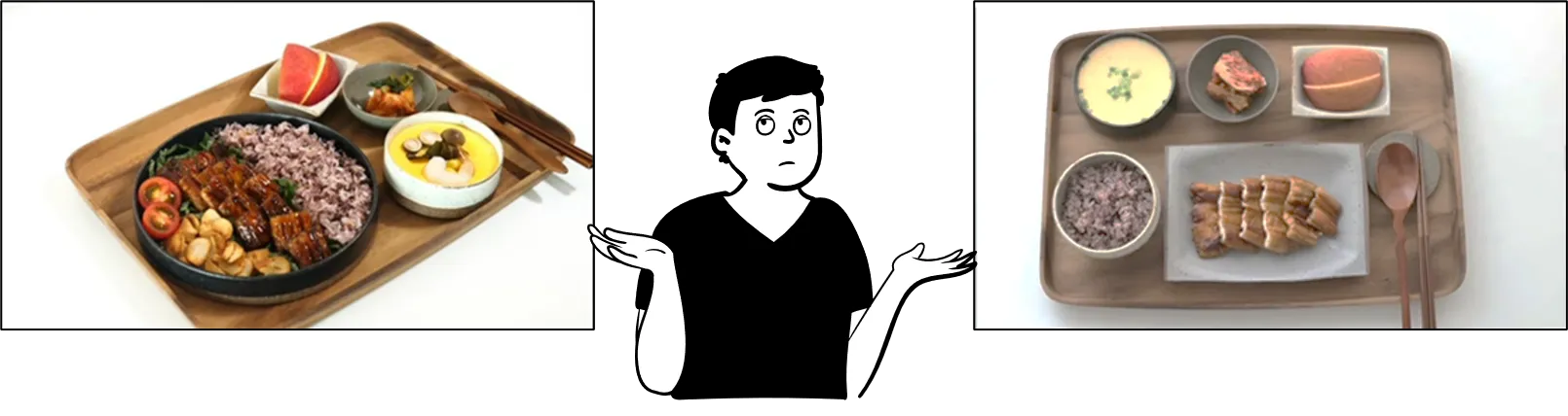
Fancy visualization of research products can be as important as attractive plating in food.

•

Even if the content is the same, how you organize and present the material can significantly influence your audience’s interest level.

1.2 Common Features of the Prestigious Journals’ Paper

•

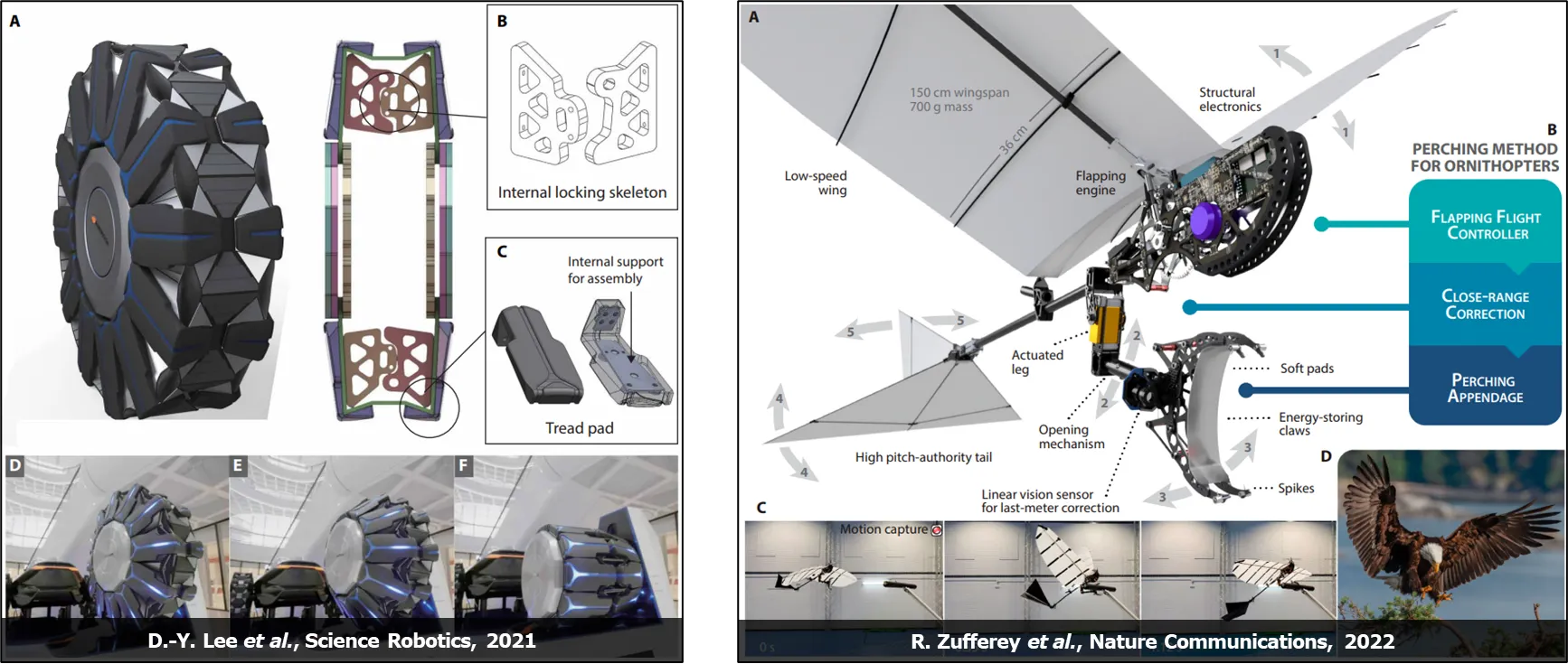
Papers published in prestigious journals like Science and Nature feature at least one fancy representative image.

•

In fact, using fancy images can have the effect of making your research product look more high-quality.

2. How to Create Animation Videos in MATLAB

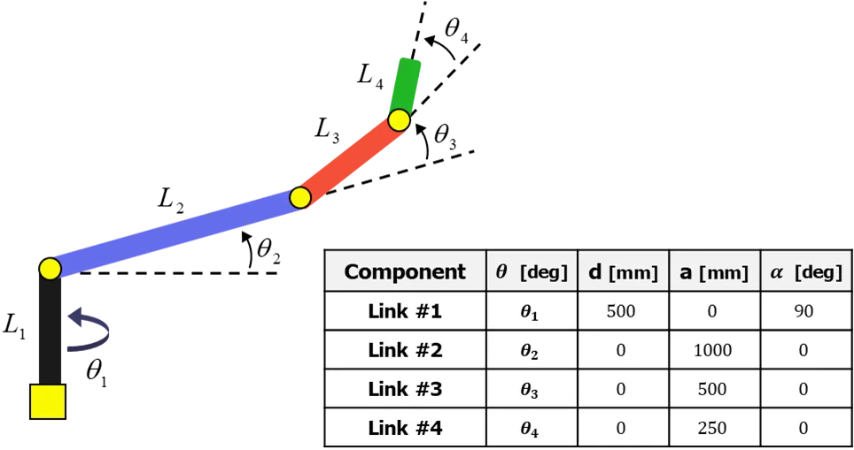
2.1 Visualization of Kinematics Results: 4-Link Robotic Arm

•

Basic Simulation Parameters

◦

Basic initialization procedures

◦

I usually keep all my MATLAB sub-functions in the “MATLAB_Function” folder and use “addpathh(genpath(’MATLAB_Function\’))” to add the folder path.

◦

By creating the time variable “t” using “Video Frame” and “Total Simulation Time”, we can easily determine the length of the final animation video.

%% Robot Arm Simulation
% H.-H. Yang (2024.08.01)


%% Initialization
close all; fclose all; clear all; clc;
rng('default'); format long;
addpath(genpath('MATLAB_Function\'));


%% Simulation Parameters
videoFrame = 30; % [fps] Video Frame
simTime = 10; % [sec] Total Simulation Time
t = linspace(0, 10, simTime*videoFrame + 1); % [sec]
t_num = length(t);
MATLAB
복사

%% Robot Arm Parameters
% Link Length
link_num = 4;
L = [500, 1000, 500, 250]; % [mm]
linkColor = {[0.1, 0.1, 0.1], [0.4, 0.4, 0.92], [0.92, 0.4, 0.4], [0.2, 0.84, 0.2]};
MATLAB
복사

•

A simple robotic arm with 4-DOF: spatial working space

•

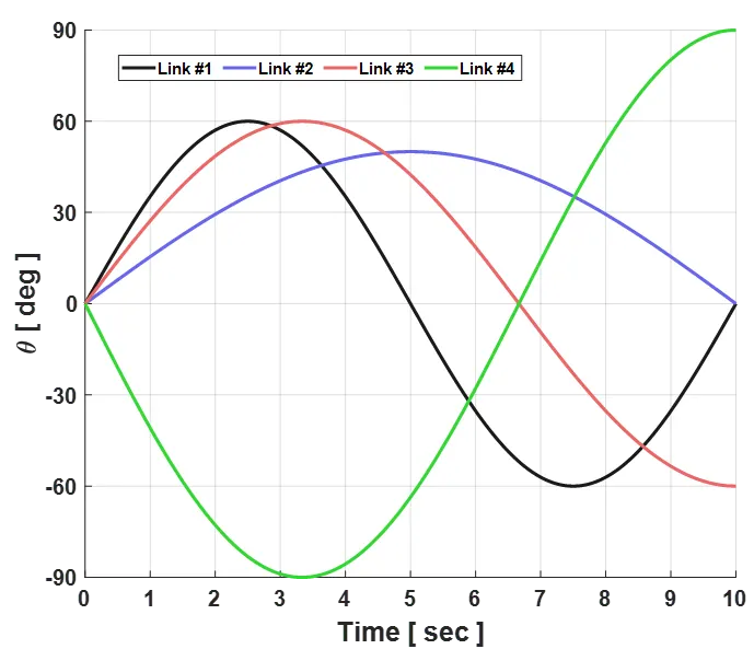
After the kinematic or dnamic analysis, we can obtain the kinematics data of each link over time.

◦

Follwing joint kinematics is assumed as the obtained kinematics results from the analysis.

%% Arbitrarily Assumed Results of the Robotic Arms' Kinematics 
% Link Joint Angle
theta1 = deg2rad(60.*sin(2.*pi.*(1/t(end)).*t)); % [rad]
del_theta1 = [0, diff(theta1)]; % [rad/s]
theta2 = deg2rad(50.*sin(2.*pi.*(0.5/t(end)).*t)); % [rad]
del_theta2 = [0, diff(theta2)]; % [rad/s]
theta3 = deg2rad(60.*sin(2.*pi.*(0.75/t(end)).*t)); % [rad]
del_theta3 = [0, diff(theta3)]; % [rad/s]
theta4 = deg2rad(-90.*sin(2.*pi.*(0.75/t(end)).*t)); % [rad]
del_theta4 = [0, diff(theta4)]; % [rad/s]
del_theta = [del_theta1; del_theta2; del_theta3; del_theta4]; % [rad]

% Plot Kinematics
[Fig, Axes] = PlotSetting(1000, 800);
xlabel('Time [ sec ]', 'FontWeight', 'bold');
ylabel('\theta [ deg ]', 'FontWeight', 'bold');
plot(t, rad2deg(theta1), '-', 'LineWidth', 3, 'Color', linkColor{1});
plot(t, rad2deg(theta2), '-', 'LineWidth', 3, 'Color', linkColor{2});
plot(t, rad2deg(theta3), '-', 'LineWidth', 3, 'Color', linkColor{3});
plot(t, rad2deg(theta4), '-', 'LineWidth', 3, 'Color', linkColor{4});
legend({'Link #1', 'Link #2', 'Link #3', 'Link #4'}, ...
        'FontSize', 15, 'Location', 'none' , 'Orientation', 'horizontal', 'NumColumns', 4);
axis([0, 10, -90, 90]);
Axes.XTick = 0:1:10; Axes.YTick = -90:30:90;
MATLAB
복사

2.2 Kinematic Animation Using “Line Geometry”

•

Line Geometry

◦

A two-point line geometry is particularly effective for visualizing simple conceptual models.

◦

Useful to show the operating process of a link mechanism

◦

The simplest way / Not suitable for perspective view

◦

Examples: Bi-Stable Gripper, Flapping Mechanism, Robotic Arm …

•

Create Animation Video

%% Kinematic Animation: Line
% Plot Setting
[Fig1, ~] = PlotSetting(1000, 800);
axis equal;
axis([-2500, 2500, -2500, 2500, -1000, 3000]);
xlabel('X [ mm ]', 'FontWeight', 'bold');
ylabel('Y [ mm ]', 'FontWeight', 'bold');
zlabel('Z [ mm ]', 'FontWeight', 'bold');
view([20, 15]);

% Link Entity (Initial Position)
linkLine{1}.geo = line([0, 0], [0, 0], [0, L(1)], 'LineWidth', 10, 'Color', linkColor{1}, 'Marker', 'o', 'MarkerSize', 10, 'MarkerFaceColor', [0.8, 0.8, 0.2]);
linkLine{2}.geo = line([0, L(2)], [0, 0], [L(1), L(1)], 'LineWidth', 5, 'Color', linkColor{2}, 'Marker', 'o', 'MarkerSize', 10, 'MarkerFaceColor', [0.8, 0.8, 0.2]);
linkLine{3}.geo = line([L(2), sum(L(2:3))], [0, 0], [L(1), L(1)], 'LineWidth', 5, 'Color', linkColor{3}, 'Marker', 'o', 'MarkerSize', 10, 'MarkerFaceColor', [0.8, 0.8, 0.2]);
linkLine{4}.geo = line([sum(L(2:3)), sum(L(2:4))], [0, 0], [L(1), L(1)], 'LineWidth', 5, 'Color', linkColor{4}, 'Marker', 'o', 'MarkerSize', 10, 'MarkerFaceColor', [0.8, 0.8, 0.2]);

% Animation Setting
video = VideoWriter('01_MATLAB\MATLAB_Line_Animation.mp4', 'MPEG-4');
video.FrameRate = videoFrame; video.Quality = 100;

% Position Analysis & Make Animation Video
open(video);
for t_idx = 1:t_num
    % Link 1 Rotation
    for link_idx = 1:link_num
        rotate(linkLine{link_idx}.geo, [0, 0, 1], rad2deg(del_theta1(t_idx)), ...
               [0, 0, 0]); 
    end
    linkLine{1}.rotAngX(t_idx) = 0.0;
    linkLine{1}.rotAngY(t_idx) = theta1(t_idx);
    linkLine{1}.rotAngZ(t_idx) = 0.0;

    % Link 2 Rotation
    rotMat2 = rotvec2mat3d(theta2(t_idx)*[0 1, 0]);
    for link_idx = 2:link_num
        rotate(linkLine{link_idx}.geo, [sin(theta1(t_idx)), -cos(theta1(t_idx)), 0], rad2deg(del_theta2(t_idx)), ...
               [linkLine{2}.geo.XData(1), linkLine{2}.geo.YData(1), linkLine{2}.geo.ZData(1)]);
    end
    linkLine{2}.rotAngX(t_idx) = theta2(t_idx);
    linkLine{2}.rotAngY(t_idx) = 0.0;
    linkLine{2}.rotAngZ(t_idx) = theta1(t_idx);

    % Link 3 Rotation
    for link_idx = 3:link_num
        rotate(linkLine{link_idx}.geo, [sin(theta1(t_idx)), -cos(theta1(t_idx)), 0], rad2deg(del_theta3(t_idx)), ...
               [linkLine{3}.geo.XData(1), linkLine{3}.geo.YData(1), linkLine{3}.geo.ZData(1)]);
    end
    linkLine{3}.rotAngX(t_idx) = theta2(t_idx) + theta3(t_idx);
    linkLine{3}.rotAngY(t_idx) = 0.0;
    linkLine{3}.rotAngZ(t_idx) = theta1(t_idx);

    % Link 4 Rotation
    rotate(linkLine{link_idx}.geo, [sin(theta1(t_idx)), -cos(theta1(t_idx)), 0], rad2deg(del_theta4(t_idx)), ...
           [linkLine{4}.geo.XData(1), linkLine{4}.geo.YData(1), linkLine{4}.geo.ZData(1)]);
    linkLine{4}.rotAngX(t_idx) = theta2(t_idx) + theta3(t_idx) + theta4(t_idx);
    linkLine{4}.rotAngY(t_idx) = 0.0;
    linkLine{4}.rotAngZ(t_idx) = theta1(t_idx);

    % Position of the Links
    for link_idx = 1:link_num
        linkLine{link_idx}.x(:,t_idx) = linkLine{link_idx}.geo.XData;
        linkLine{link_idx}.y(:,t_idx) = linkLine{link_idx}.geo.YData;
        linkLine{link_idx}.z(:,t_idx) = linkLine{link_idx}.geo.ZData;
    end

    % Position Vectors
    for link_idx = 1:link_num
        linkLine{link_idx}.r(:,t_idx) = [linkLine{link_idx}.geo.XData(2); linkLine{link_idx}.geo.YData(2); linkLine{link_idx}.geo.ZData(2)] ...
                                        - [linkLine{link_idx}.geo.XData(1); linkLine{link_idx}.geo.YData(1); linkLine{link_idx}.geo.ZData(1)];
    end

    % Write Video
    drawnow; frame = getframe(Fig1); writeVideo(video, frame);
end
close(video);
MATLAB
복사

•

Results

◦

We can roughly understand the motion of the robotic arm.

◦

It shows a lack of perspective in 3D animation due to the limitation of MATLAB line geometry.

2.3 Kinematic Animation Using “Simple Patch Geometry”

•

Simple Patch Geometry

◦

The patch geometry is typically used to visualize a general surface structure by defining the faces and vertices of the patch.

◦

The best way to visualize the conceptual model

◦

A little tricky pre-processing to create patch geometry

◦

Examples: Wake Pattern, Origami Structure, Deployable Structure …

•

Simple Patch of 4-Link Robotic Arm

◦

Assume all link shapes are rectangular

function [Patch_Faces, Patch_Vertices] = ImportRobotArmPatchData
% Link 1
w = 200; l = 500; offset = [0, 0, 0];
Patch_Faces{1} = [1, 2, 3, 4; 1, 5, 6, 2; 2, 6, 7, 3; 3, 7, 8, 4; 4, 8, 5, 1; 5, 6, 7, 8];
Patch_Vertices{1} = [-0.5*w, -0.5*w, 0; -0.5*w, 0.5*w, 0; 0.5*w, 0.5*w, 0; 0.5*w, -0.5*w, 0; ...
                   -0.5*w, -0.5*w, l; -0.5*w, 0.5*w, l; 0.5*w, 0.5*w, l; 0.5*w, -0.5*w, l;];
Patch_Vertices{1} = Patch_Vertices{1} + repmat(offset, 8, 1);

% Link 2
w = 100; l = 1000; offset = [0, 0, 500];
Patch_Faces{2} = [1, 2, 3, 4; 1, 5, 6, 2; 2, 6, 7, 3; 3, 7, 8, 4; 4, 8, 5, 1; 5, 6, 7, 8];
Patch_Vertices{2} = [0, -0.5*w, -0.5*w; 0, 0.5*w, -0.5*w; l, 0.5*w, -0.5*w; l, -0.5*w, -0.5*w; ...
                     0, -0.5*w, 0.5*w; 0, 0.5*w, 0.5*w; l, 0.5*w, 0.5*w; l, -0.5*w, 0.5*w];
Patch_Vertices{2} = Patch_Vertices{2} + repmat(offset, 8, 1);

% Link 3
w = 150; l = 500; offset = [1000, 0, 500];
Patch_Faces{3} = [1, 2, 3, 4; 1, 5, 6, 2; 2, 6, 7, 3; 3, 7, 8, 4; 4, 8, 5, 1; 5, 6, 7, 8];
Patch_Vertices{3} = [0, -0.5*w, -0.5*w; 0, 0.5*w, -0.5*w; l, 0.5*w, -0.5*w; l, -0.5*w, -0.5*w; ...
                     0, -0.5*w, 0.5*w; 0, 0.5*w, 0.5*w; l, 0.5*w, 0.5*w; l, -0.5*w, 0.5*w];
Patch_Vertices{3} = Patch_Vertices{3} + repmat(offset, 8, 1);

% Link 4
w = 200; l = 250; offset = [1500, 0, 500];
Patch_Faces{4} = [1, 2, 3, 4; 1, 5, 6, 2; 2, 6, 7, 3; 3, 7, 8, 4; 4, 8, 5, 1; 5, 6, 7, 8];
Patch_Vertices{4} = [0, -0.5*w, -0.5*w; 0, 0.5*w, -0.5*w; l, 0.5*w, -0.5*w; l, -0.5*w, -0.5*w; ...
                     0, -0.5*w, 0.5*w; 0, 0.5*w, 0.5*w; l, 0.5*w, 0.5*w; l, -0.5*w, 0.5*w];
Patch_Vertices{4} = Patch_Vertices{4} + repmat(offset, 8, 1);
MATLAB
복사

•

Create Animation Video

%% Kinematicc Animation: Simple Patch
% Robotic Arm's Patch Data (User Defined Simple Patch Data)
[Patch_Faces, Patch_Vertices] = ImportRobotArmPatchData;

% Plot Setting
[Fig2, Axes2] = PlotSetting(1000, 800);
axis equal;
axis([-2500, 2500, -2500, 2500, -1000, 3000]);
xlabel('X [ mm ]', 'FontWeight', 'bold');
ylabel('Y [ mm ]', 'FontWeight', 'bold');
zlabel('Z [ mm ]', 'FontWeight', 'bold');
view([20, 15]);

% link Entity (Initial Position): Low-Quality
linkPatch = cell(1,link_num);
for link_idx = 1:link_num
    linkPatch{link_idx}.geo = patch('Faces', Patch_Faces{link_idx}, 'Vertices', Patch_Vertices{link_idx}, ...
                                    'FaceColor', linkColor{link_idx}, 'EdgeColor', [0, 0, 0], 'FaceAlpha', 1.0);
end

% Animation Setting
video = VideoWriter('01_MATLAB\MATLAB_Patch_Animation.mp4', 'MPEG-4');
video.FrameRate = videoFrame;

% Position Analysis & Make Animation Video
open(video);
for t_idx = 1:t_num
    % Link 1 Rotation
    for link_idx = 1:link_num
        rotate(linkPatch{link_idx}.geo, [0, 0, 1], rad2deg(del_theta1(t_idx)), ...
               [linkLine{1}.x(1,t_idx), linkLine{1}.y(1,t_idx), linkLine{1}.z(1,t_idx)]);
    end

    % Link 2 Rotation
    for link_idx = 2:link_num
        rotate(linkPatch{link_idx}.geo, [sin(theta1(t_idx)), -cos(theta1(t_idx)), 0], rad2deg(del_theta2(t_idx)), ...
               [linkLine{2}.x(1,t_idx), linkLine{2}.y(1,t_idx), linkLine{2}.z(1,t_idx)]);
    end
    
    % Link 3 Rotation
    for link_idx = 3:link_num
        rotate(linkPatch{link_idx}.geo, [sin(theta1(t_idx)), -cos(theta1(t_idx)), 0], rad2deg(del_theta3(t_idx)), ...
               [linkLine{3}.x(1,t_idx), linkLine{3}.y(1,t_idx), linkLine{3}.z(1,t_idx)]);
    end

    % Link 4 Rotation
    rotate(linkPatch{link_idx}.geo, [sin(theta1(t_idx)), -cos(theta1(t_idx)), 0], rad2deg(del_theta4(t_idx)), ...
           [linkLine{4}.x(1,t_idx), linkLine{4}.y(1,t_idx), linkLine{4}.z(1,t_idx)]);

    % Write Video
    drawnow; frame = getframe(Fig2); writeVideo(video, frame);
end
close(video);
MATLAB
복사

•

Results

◦

By using the patch geometry, we can create a more intuitive animation video for the robotic arm.

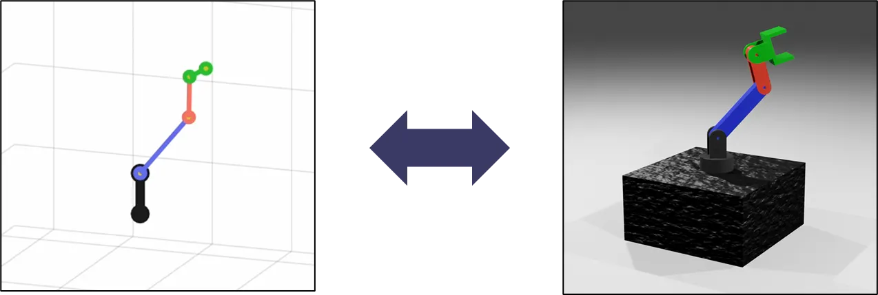
2.4 Kinematic Animation Using “CAD Patch Geometry”

•

CAD Patch Geometry

◦

We can import the CAD model geometry into MATLAB as patch data if you have a CAD model.

◦

The animation video with CAD patch geometry give you a complete understadning of the model’s behavior.

•

How to Import the CAD Model

◦

The “importGeometry“ function is used to get the CAD model geometry data, and the “scale” function is used to match the unit scale properly.

◦

The “pdegplot” function plots the CAD geometry.

◦

The geometry data, such as faces, vertices, and lines, are stored in other variables to utilize for the animation video.

function [CADGeo_Faces, CADGeo_Vertices, CADGeo_Lines] = ImportRobotArmCAD(link_num)
% Pre-Allocation
CADGeo_Faces = cell(1,link_num);
CADGeo_Vertices = cell(1,link_num);
CADGeo_Lines = cell(1,link_num);

% CAD Model (STEP File)
[Fig, ~] = PlotSetting(100, 100);
for link_idx = 1:link_num
    CADModelPath = ['Input\Link', num2str(link_idx), '.stp'];
    CADModel = importGeometry(CADModelPath); % [m]
    CADModel = scale(CADModel, [1000, 1000, 1000]); % [mm]
    CADGeo = pdegplot(CADModel);
    CADGeo_Faces{link_idx} = CADGeo(1).Faces;
    CADGeo_Vertices{link_idx} = CADGeo(1).Vertices;
    CADGeo_Lines{link_idx}.XData = CADGeo(2).XData;
    CADGeo_Lines{link_idx}.YData = CADGeo(2).YData;
    CADGeo_Lines{link_idx}.ZData = CADGeo(2).ZData;
end
close(Fig);
MATLAB
복사

•

Create Animation Video

%% Kinematic Animation: CAD Patch Geometry
% Robotic Arm's Patch Data (CAD Model Data)
[CADGeo_Faces, CADGeo_Vertices, CADGeo_Lines] = ImportRobotArmCAD(link_num);

% Plot Setting 1
[Fig3, Axes3] = PlotSetting(1000, 800);
axis equal;
axis([-2500, 2500, -2500, 2500, -1000, 3000]);
xlabel('X [ mm ]', 'FontWeight', 'bold');
ylabel('Y [ mm ]', 'FontWeight', 'bold');
zlabel('Z [ mm ]', 'FontWeight', 'bold');
view([20, 15]);

% link Entity (Initial Position): Low-Quality
linkCAD1 = cell(1,link_num);
for link_idx = 1:link_num
    linkCAD1{link_idx}.geo = patch('Faces', CADGeo_Faces{link_idx}, 'Vertices', CADGeo_Vertices{link_idx}, ...
                                   'FaceColor', linkColor{link_idx}, 'EdgeColor', 'none', 'FaceAlpha', 1.0);
    linkCAD1{link_idx}.line = line(CADGeo_Lines{link_idx}.XData, CADGeo_Lines{link_idx}.YData, CADGeo_Lines{link_idx}.ZData, ...
                                   'LineWidth', 0.1, 'Color', [0, 0, 0]);
end

% Animation Setting
video = VideoWriter('01_MATLAB\MATLAB_CAD_Animation_Default.mp4', 'MPEG-4');
video.FrameRate = videoFrame;

% Position Analysis & Make Animation Video
open(video);
for t_idx = 1:t_num
    % Link 1 Rotation
    for link_idx = 1:link_num
        rotate(linkCAD1{link_idx}.geo, [0, 0, 1], rad2deg(del_theta1(t_idx)), ...
               [linkLine{1}.x(1,t_idx), linkLine{1}.y(1,t_idx), linkLine{1}.z(1,t_idx)]);
        rotate(linkCAD1{link_idx}.line, [0, 0, 1], rad2deg(del_theta1(t_idx)), ...
               [linkLine{1}.x(1,t_idx), linkLine{1}.y(1,t_idx), linkLine{1}.z(1,t_idx)]);
    end

    % Link 2 Rotation
    for link_idx = 2:link_num
        rotate(linkCAD1{link_idx}.geo, [sin(theta1(t_idx)), -cos(theta1(t_idx)), 0], rad2deg(del_theta2(t_idx)), ...
               [linkLine{2}.x(1,t_idx), linkLine{2}.y(1,t_idx), linkLine{2}.z(1,t_idx)]);
        rotate(linkCAD1{link_idx}.line, [sin(theta1(t_idx)), -cos(theta1(t_idx)), 0], rad2deg(del_theta2(t_idx)), ...
               [linkLine{2}.x(1,t_idx), linkLine{2}.y(1,t_idx), linkLine{2}.z(1,t_idx)]);
    end
    
    % Link 3 Rotation
    for link_idx = 3:link_num
        rotate(linkCAD1{link_idx}.geo, [sin(theta1(t_idx)), -cos(theta1(t_idx)), 0], rad2deg(del_theta3(t_idx)), ...
               [linkLine{3}.x(1,t_idx), linkLine{3}.y(1,t_idx), linkLine{3}.z(1,t_idx)]);
        rotate(linkCAD1{link_idx}.line, [sin(theta1(t_idx)), -cos(theta1(t_idx)), 0], rad2deg(del_theta3(t_idx)), ...
               [linkLine{3}.x(1,t_idx), linkLine{3}.y(1,t_idx), linkLine{3}.z(1,t_idx)]);
    end

    % Link 4 Rotation
    rotate(linkCAD1{link_idx}.geo, [sin(theta1(t_idx)), -cos(theta1(t_idx)), 0], rad2deg(del_theta4(t_idx)), ...
           [linkLine{4}.x(1,t_idx), linkLine{4}.y(1,t_idx), linkLine{4}.z(1,t_idx)]);
    rotate(linkCAD1{link_idx}.line, [sin(theta1(t_idx)), -cos(theta1(t_idx)), 0], rad2deg(del_theta4(t_idx)), ...
           [linkLine{4}.x(1,t_idx), linkLine{4}.y(1,t_idx), linkLine{4}.z(1,t_idx)]);

    % Write Video
    drawnow; frame = getframe(Fig3); writeVideo(video, frame);
end
close(video);

% Plot Setting 2
[Fig4, Axes4] = PlotSetting(1000, 800);
axis equal;
axis([-2500, 2500, -2500, 2500, -1000, 3000]);
xlabel('X [ mm ]', 'FontWeight', 'bold');
ylabel('Y [ mm ]', 'FontWeight', 'bold');
zlabel('Z [ mm ]', 'FontWeight', 'bold');

% Light Option
light('Style', 'local', 'Position', [0, 0, 5000]);
light('Style', 'local', 'Position', [5000, -5000, 5000]);

% View Option
view([80, 25]);
view_t1_idxSet = 1:round(0.5*t_num); view_t1_num = length(view_t1_idxSet);
view_t2_idxSet = round(0.5*t_num):t_num; view_t2_num = length(view_t2_idxSet);
view_az(view_t1_idxSet) = linspace(80, 60, view_t1_num);
view_az(view_t2_idxSet) = linspace(60, 20, view_t2_num);
view_el(view_t1_idxSet) = linspace(25, 25, view_t1_num);
view_el(view_t2_idxSet) = linspace(25, 15, view_t2_num);

% Axes Tick Option
axesTick = -5000:1000:5000;
Axes4.XTick = axesTick; Axes4.YTick = axesTick; Axes4.ZTick = axesTick;
Axes4.XTickLabelRotation = 0; Axes4.YTickLabelRotation = 0; Axes4.ZTickLabelRotation = 0;
Axes4.TickDir = 'in';
Axes4.TickLength = [0.01, 0.01];

% Ground
ground_Faces = [1, 2, 3, 4; 1, 5, 6, 2; 2, 6, 7, 3; 3, 7, 8, 4; 4, 8, 5, 1; 5, 6, 7, 8];
ground_Vertices = [-1000, -1000, 0; -1000, 1000, 0; 1000, 1000, 0; 1000, -1000, 0; ...
                   -1000, -1000, -1000; -1000, 1000, -1000; 1000, 1000, -1000; 1000, -1000, -1000;];
ground = patch('Faces', ground_Faces, 'Vertices', ground_Vertices, ...
               'FaceColor', [0.25, 0.25, 0.25], 'EdgeColor', [0.0, 0.0, 0.0], 'FaceAlpha', 0.9);

% link Entity (Initial Position): High-Quality
linkCAD2 = cell(1,link_num);
for link_idx = 1:link_num
    linkCAD2{link_idx}.geo = patch('Faces', CADGeo_Faces{link_idx}, 'Vertices', CADGeo_Vertices{link_idx}, ...
                                   'FaceColor', linkColor{link_idx}, 'EdgeColor', 'none', 'FaceAlpha', 1.0);
    linkCAD2{link_idx}.geo.FaceLighting = 'gouraud'; % flat / gouraud / none
    linkCAD2{link_idx}.geo.BackFaceLighting = 'reverselit'; % reverselit / unlit / lit
    linkCAD2{link_idx}.geo.AmbientStrength = 0.4; % 0.3 [0, 1]
    linkCAD2{link_idx}.geo.DiffuseStrength = 0.8; % 0.6 [0, 1]
    linkCAD2{link_idx}.geo.SpecularStrength = 0.8; % 0.9 [0, 1]
    linkCAD2{link_idx}.geo.SpecularExponent = 20; % 10 [5, 20]
    linkCAD2{link_idx}.line = line(CADGeo_Lines{link_idx}.XData, CADGeo_Lines{link_idx}.YData, CADGeo_Lines{link_idx}.ZData, ...
                                    'LineWidth', 0.1, 'Color', [0, 0, 0]);
end

% Animation Setting
video = VideoWriter('01_MATLAB\MATLAB_CAD_Animation_Rev.mp4', 'MPEG-4');
video.FrameRate = videoFrame; video.Quality = 100;

% Position Analysis & Make Animation Video
open(video);
for t_idx = 1:t_num
    % Link 1 Rotation
    for link_idx = 1:link_num
        rotate(linkCAD2{link_idx}.geo, [0, 0, 1], rad2deg(del_theta1(t_idx)), ...
               [linkLine{1}.x(1,t_idx), linkLine{1}.y(1,t_idx), linkLine{1}.z(1,t_idx)]);
        rotate(linkCAD2{link_idx}.line, [0, 0, 1], rad2deg(del_theta1(t_idx)), ...
               [linkLine{1}.x(1,t_idx), linkLine{1}.y(1,t_idx), linkLine{1}.z(1,t_idx)]);
    end

    % Link 2 Rotation
    for link_idx = 2:link_num
        rotate(linkCAD2{link_idx}.geo, [sin(theta1(t_idx)), -cos(theta1(t_idx)), 0], rad2deg(del_theta2(t_idx)), ...
               [linkLine{2}.x(1,t_idx), linkLine{2}.y(1,t_idx), linkLine{2}.z(1,t_idx)]);
        rotate(linkCAD2{link_idx}.line, [sin(theta1(t_idx)), -cos(theta1(t_idx)), 0], rad2deg(del_theta2(t_idx)), ...
               [linkLine{2}.x(1,t_idx), linkLine{2}.y(1,t_idx), linkLine{2}.z(1,t_idx)]);
    end
    
    % Link 3 Rotation
    for link_idx = 3:link_num
        rotate(linkCAD2{link_idx}.geo, [sin(theta1(t_idx)), -cos(theta1(t_idx)), 0], rad2deg(del_theta3(t_idx)), ...
               [linkLine{3}.x(1,t_idx), linkLine{3}.y(1,t_idx), linkLine{3}.z(1,t_idx)]);
        rotate(linkCAD2{link_idx}.line, [sin(theta1(t_idx)), -cos(theta1(t_idx)), 0], rad2deg(del_theta3(t_idx)), ...
               [linkLine{3}.x(1,t_idx), linkLine{3}.y(1,t_idx), linkLine{3}.z(1,t_idx)]);
    end

    % Link 4 Rotation
    rotate(linkCAD2{link_idx}.geo, [sin(theta1(t_idx)), -cos(theta1(t_idx)), 0], rad2deg(del_theta4(t_idx)), ...
           [linkLine{4}.x(1,t_idx), linkLine{4}.y(1,t_idx), linkLine{4}.z(1,t_idx)]);
    rotate(linkCAD2{link_idx}.line, [sin(theta1(t_idx)), -cos(theta1(t_idx)), 0], rad2deg(del_theta4(t_idx)), ...
           [linkLine{4}.x(1,t_idx), linkLine{4}.y(1,t_idx), linkLine{4}.z(1,t_idx)]);

    % Change View
    view(view_az(t_idx), view_el(t_idx));

    % Write Video
    drawnow; frame = getframe(Fig4); writeVideo(video, frame);
end
close(video);
MATLAB
복사

•

Results

◦

By using the CAD patch geometry, we can clearly understand the robotic arm’s motion during the simulation time.

◦

In addition, we can also create a more dynamic animation by adjusting the light and view control options.

Whole MATLAB scripts are attached in “Robotic_Arm_MATLAB_Animation.zip”.

Robotic_Arm_MATLAB_Animation.zip

255.0KB

3. Other Visualization Tools

3.1 Blender

•

Blender Animation Using Python Script & Prescribed Kinematic Input Data

◦

We can automate all tasks in Blender via Python script: importing CAD model, applying materials …

◦

We can apply the kinematics data obtained from MATLAB to the importing CAD models by writing proper input files.

3.2 KeyShot

•

KeyShot Animation for Promotion Video

◦

We can create a fancy animation video using KeyShot

If you’d like to learn more about how to use the other visualization tools (Blender, KeyShot, Unreal Engine), feel free to contact me!

Go Top of Page